
手写数字识别
使用 MLP 实现
设置
1 | import tensorflow as tf |
[PhysicalDevice(name='/physical_device:GPU:0', device_type='GPU')]载入数据
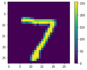
1 | (x_train,y_train),(x_test,y_test) = mnist.load_data() |

load_data()
返回:
两个元组:
x_train, x_test: uint8 数组表示的灰度图像,尺寸为 (num_samples, 28, 28)

y_train, y_test: uint8 数组表示的数字标签(范围在 0-9 之间的整数),尺寸为 (num_samples,)参数: path: 如果在本地没有索引文件 (at '~/.keras/datasets/' + path), 它将被下载到该目录
Mnist 数据集
训练集为 60,000 张 28x28 像素灰度图像,测试集为 10,000 同规格图像,总共 10 类数字标签。
处理原始数据
1 |
|
(60000, 28, 28) train data
(10000, 28, 28) test data将原始数据归一化。归一化的作用
转换标签
1 | from keras.utils import to_categorical |
[[0. 0. 0. ... 1. 0. 0.]
 [0. 0. 1. ... 0. 0. 0.]
 [0. 1. 0. ... 0. 0. 0.]
 ...
 [0. 0. 0. ... 0. 0. 0.]
 [0. 0. 0. ... 0. 0. 0.]
 [0. 0. 0. ... 0. 0. 0.]]
使用 to_categorical() 将标签向量转化为 binary matrix
构建模型
1 | from keras.models import Sequential |
Model: "sequential"
_________________________________________________________________
Layer (type)                 Output Shape              Param #
=================================================================
flatten (Flatten)            (None, 784)               0
_________________________________________________________________
Dense1 (Dense)               (None, 512)               401920
_________________________________________________________________
dropout1 (Dropout)           (None, 512)               0
_________________________________________________________________
Dense2 (Dense)               (None, 128)               65664
_________________________________________________________________
dropout2 (Dropout)           (None, 128)               0
_________________________________________________________________
softmax (Dense)              (None, 10)                1290
=================================================================
Total params: 468,874
Trainable params: 468,874
Non-trainable params: 0
_________________________________________________________________
网络第一层 Flatten 将图像转换成以为数组,该层没有要学习的参数。
每个 Dense 层有 512 神经元, 最后一个使用 softmax 激活函数,它可以将一个数值向量归一化为一个概率分布向量:
\[ Softmax(zi) = \frac{e^{z_i}}{\sum_j {e^{z_j}}} \]
编译模型
1 | from keras.losses import categorical_crossentropy |
使用 Admax 优化器,categotical_crossentropy(交叉熵损失) 作为损失函数,通常与 softmax 配合使用:
\[ Loss = -log(1-p_i) \]
\(p_i\)是预测样本真实标签得到的概率
训练模型
调用 model.fit 方法,这样命名因为会将模型与训练数据进行拟合
1 | model.fit(x_train,y_train,batch_size=128,epochs=10,verbose=1,validation_data=(x_test,y_test)) |
Epoch 1/10
469/469 [==============================] - 4s 5ms/step - loss: 0.7144 - accuracy: 0.7838 - val_loss: 0.1901 - val_accuracy: 0.9447
Epoch 2/10
469/469 [==============================] - 2s 4ms/step - loss: 0.2355 - accuracy: 0.9317 - val_loss: 0.1319 - val_accuracy: 0.9605
Epoch 3/10
469/469 [==============================] - 2s 4ms/step - loss: 0.1644 - accuracy: 0.9515 - val_loss: 0.1056 - val_accuracy: 0.9678
Epoch 4/10
469/469 [==============================] - 2s 4ms/step - loss: 0.1290 - accuracy: 0.9617 - val_loss: 0.0917 - val_accuracy: 0.9717
Epoch 5/10
469/469 [==============================] - 2s 4ms/step - loss: 0.1077 - accuracy: 0.9687 - val_loss: 0.0837 - val_accuracy: 0.9743
Epoch 6/10
469/469 [==============================] - 2s 4ms/step - loss: 0.0963 - accuracy: 0.9710 - val_loss: 0.0751 - val_accuracy: 0.9759
Epoch 7/10
469/469 [==============================] - 2s 4ms/step - loss: 0.0802 - accuracy: 0.9763 - val_loss: 0.0738 - val_accuracy: 0.9772
Epoch 8/10
469/469 [==============================] - 2s 4ms/step - loss: 0.0714 - accuracy: 0.9790 - val_loss: 0.0663 - val_accuracy: 0.9791
Epoch 9/10
469/469 [==============================] - 2s 4ms/step - loss: 0.0664 - accuracy: 0.9798 - val_loss: 0.0647 - val_accuracy: 0.9798
Epoch 10/10
469/469 [==============================] - 2s 4ms/step - loss: 0.0570 - accuracy: 0.9830 - val_loss: 0.0633 - val_accuracy: 0.9800
epochs 是训练次数,validation_date 是划分出测试集,训练集正确率达到98%以上
评估准确率
1 | test_loss,test_acc = model.evaluate(x_test,y_test,verbose=1) |
313/313 [==============================] - 1s 2ms/step - loss: 0.0284 - accuracy: 0.9916

Test accurancy 0.991599977016449
进行预测
来看第一个预测结果
1 | import numpy as np |
7可以绘制图表,查看对全部类的预测
1 | def plot_image(i,predictions_array, true_label, img): |
正确标签为蓝色,错误为红色
验证预测结果
1 | num_rows = 10 |

使用 CNN
重新载入数据
1 | (x_train,y_train),(x_test,y_test) = mnist.load_data() |
x.shape = (samples_nums, height, width, channels)
构建模型
1 | from keras.layers import Conv2D,MaxPooling2D |
Model: "sequential_5"
_________________________________________________________________
Layer (type)                 Output Shape              Param #
=================================================================
conv2d_8 (Conv2D)            (None, 26, 26, 32)        320
_________________________________________________________________
dropout_12 (Dropout)         (None, 26, 26, 32)        0
_________________________________________________________________
conv2d_9 (Conv2D)            (None, 24, 24, 16)        4624
_________________________________________________________________
max_pooling2d_4 (MaxPooling2 (None, 12, 12, 16)        0
_________________________________________________________________
dropout_13 (Dropout)         (None, 12, 12, 16)        0
_________________________________________________________________
flatten_5 (Flatten)          (None, 2304)              0
_________________________________________________________________
dense_8 (Dense)              (None, 128)               295040
_________________________________________________________________
dropout_14 (Dropout)         (None, 128)               0
_________________________________________________________________
dense_9 (Dense)              (None, 10)                1290
=================================================================
Total params: 301,274
Trainable params: 301,274
Non-trainable params: 0
_________________________________________________________________
编译和训练模型
选择 Adamdelta 作为优化器
1 | from keras.optimizers import Adam |
Epoch 1/10
469/469 [==============================] - 6s 9ms/step - loss: 0.6243 - accuracy: 0.8000 - val_loss: 0.0790 - val_accuracy: 0.9767
Epoch 2/10
469/469 [==============================] - 3s 7ms/step - loss: 0.1273 - accuracy: 0.9605 - val_loss: 0.0503 - val_accuracy: 0.9837
Epoch 3/10
469/469 [==============================] - 3s 6ms/step - loss: 0.0927 - accuracy: 0.9715 - val_loss: 0.0396 - val_accuracy: 0.9874
Epoch 4/10
469/469 [==============================] - 3s 7ms/step - loss: 0.0748 - accuracy: 0.9758 - val_loss: 0.0387 - val_accuracy: 0.9891
Epoch 5/10
469/469 [==============================] - 3s 6ms/step - loss: 0.0634 - accuracy: 0.9814 - val_loss: 0.0355 - val_accuracy: 0.9880
Epoch 6/10
469/469 [==============================] - 3s 7ms/step - loss: 0.0558 - accuracy: 0.9828 - val_loss: 0.0331 - val_accuracy: 0.9900
Epoch 7/10
469/469 [==============================] - 3s 6ms/step - loss: 0.0502 - accuracy: 0.9835 - val_loss: 0.0295 - val_accuracy: 0.9911
Epoch 8/10
469/469 [==============================] - 3s 6ms/step - loss: 0.0488 - accuracy: 0.9848 - val_loss: 0.0296 - val_accuracy: 0.9906
Epoch 9/10
469/469 [==============================] - 3s 6ms/step - loss: 0.0439 - accuracy: 0.9856 - val_loss: 0.0313 - val_accuracy: 0.9910
Epoch 10/10
469/469 [==============================] - 3s 6ms/step - loss: 0.0420 - accuracy: 0.9865 - val_loss: 0.0303 - val_accuracy: 0.9912

<tensorflow.python.keras.callbacks.History at 0x16d0c5fa340>
评估准确率
1 | test_loss, test_acc = model.evaluate(x_test, y_test, verbose= 2) |
313/313 - 1s - loss: 0.0303 - accuracy: 0.9912

Test accuracy: 0.9911999702453613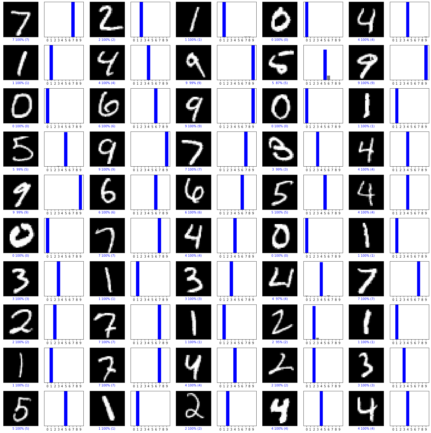
CNN 与 MLP 对比
- CNN 能提取像素间的空间关系,而 MLP 将图像变为一维向量丢失空间信息
- MLP 是每一层是全连接的,参数数量多, CNN 每一层共享 kernel ,节点之间不是全连接,因此参数大小取决于 kernel 大小,参数数量少
- CNN 具有 局部平移不变性, 即无论图像出现在那个位置,都能提取到该特征。(因为共享 filter). 而 MLP 不具有平移不变性,如果一张图片的特征出现在左上,而另一张特征出现在右下,那么 MLP 将尝试往右下修正参数。